When you purchase through links on our site, we may earn an affiliate commission.Heres how it works.
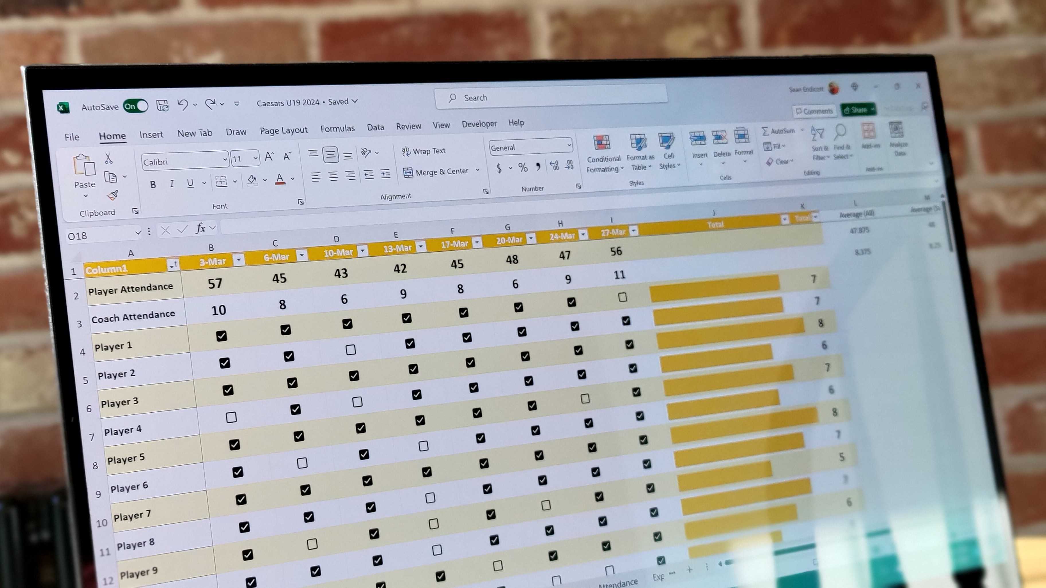
Ever find yourself with aMicrosoft Excelspreadsheet jam-packed full of data but don’t know where to look next?
Do you wish you could sift, sort, and analyze and make your data work harder for you?

Well, look no further.
Although we have only provided 7 tools here, they will make a huge difference to your capabilities.
Most of these tools are relatively basic, but a few of the later ones may border on intermediate.
So without further ado, let’s look at our first simple tool to get your data working.
Sum
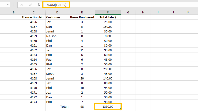
Its as simple as it sounds.
Use the Sum function to Sum (add up) all of the requested data.
you might do this across rows or columns, even adding together multiple numerical sources on your spreadsheet.
Still a simple tool, but much more functional than it first appears.
Count
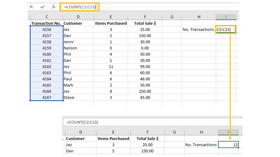
The most basic Count function does exactly what it says.
It counts the total number of cells highlighted in a range.
A range can be across multiple rows and columns, like A1:A50 or A1:D50.
The above example shows the total number of transactions made by customers in a small database.
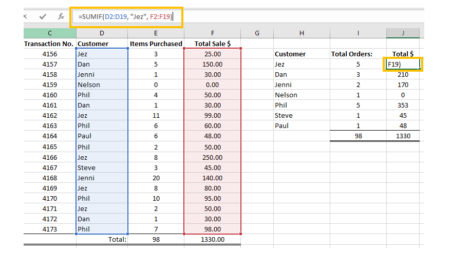
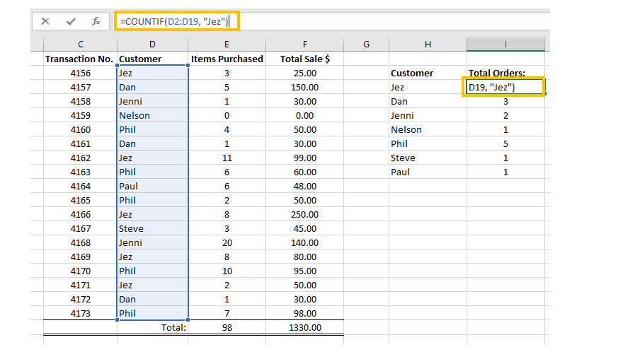
To do this, the formula would be =CountIf(F1:F19, >100).
One difference you will notice is the inclusion of [sum_range] in the formula.
This lets us specify the rules in one column but add the values from another corresponding column.
or
This little tool can be a real time saver.
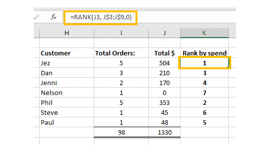
This is done using the rank formula.
Our above example shows which of our customers are making the most / least expenditure on sales.
Vlookup
The infamous VLookup is extremely useful but not nearly as difficult as its reputation suggests.
The formula used for this is:
Although this looks complicated at first, it’s actually quite straightforward.
Let’s break it down:
Lookup_valueis the cell it reads before it goes off searching.
This is a unique string of information you pop in to prompt the search.
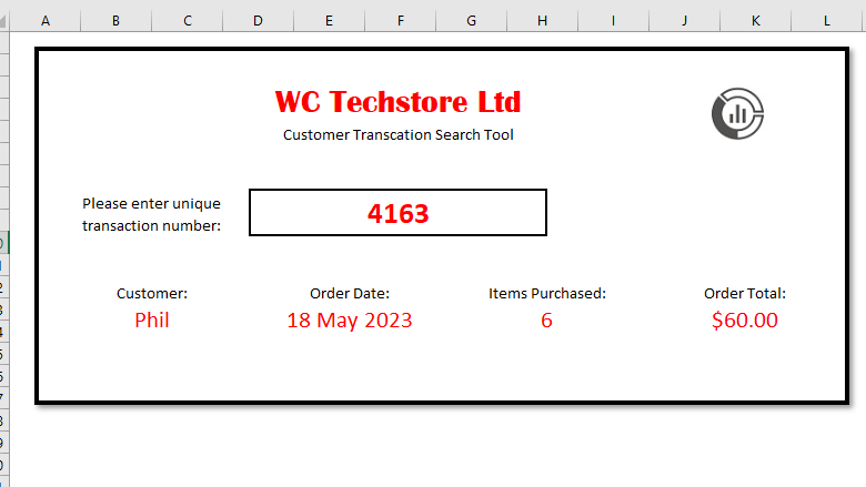
For example, you might throw in in a transaction number to look up a specific customer sale.
Table_arrayis the search location.
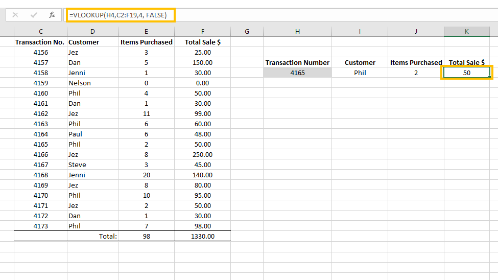
Your unique lookup_value should always be in the first column in this table.
Col_index_numis the column from the above Table_array, which will provide you with the data to output.
Range_lookupis an optional field.
Here you might enter either TRUE or FALSE.
If TRUE, then the lookup will search for an approximate match.
If FALSE, then the lookup wants an exact match.

If left blank, this will always default to TRUE.
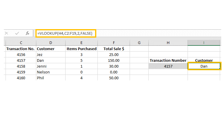
In the example, the VLOOKUP formula in cell I4 reads the transaction number from cell H4.
It then reads across to this column and sends back the name Dan.

You only need to change the column number to look at the adjacent information to pull that through too.
As useful as they are, Vlookups do come with a couple of limitations.
Firstly, the VLookup value will not recognize any duplicate values.

Secondly, Vlookups can only look right.
This isn’t a Zoolander reference but a feature of how the search works.
There are way around this, such as the XLOOKUP function, but they are a bit more advanced.

Your data can keep you informed and save precious hours, all whilst looking good at the same time.